Screenshots
Project deep-dive
Video or photos → metric-scaled 3D. · A testbed for CV and VLM ideas.
Three scene modes. Fourteen stages. Fully automated — video or stills in, dense point cloud, mesh, and Gaussian splat out. Built as a research platform, not a product. Fork it. Swap a stage. Answer your own question. Six VLM integrations were tried here. The findings are documented.
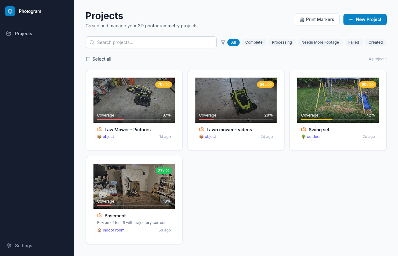
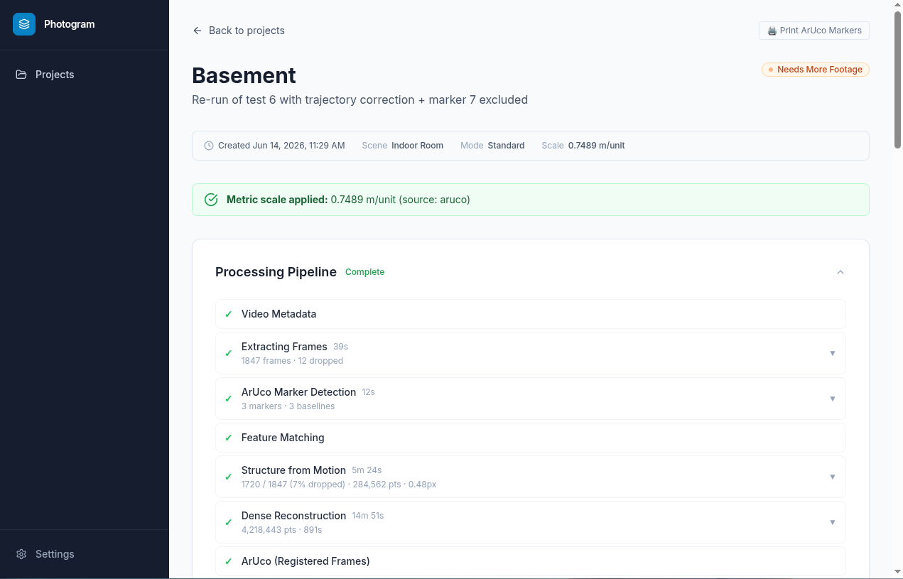
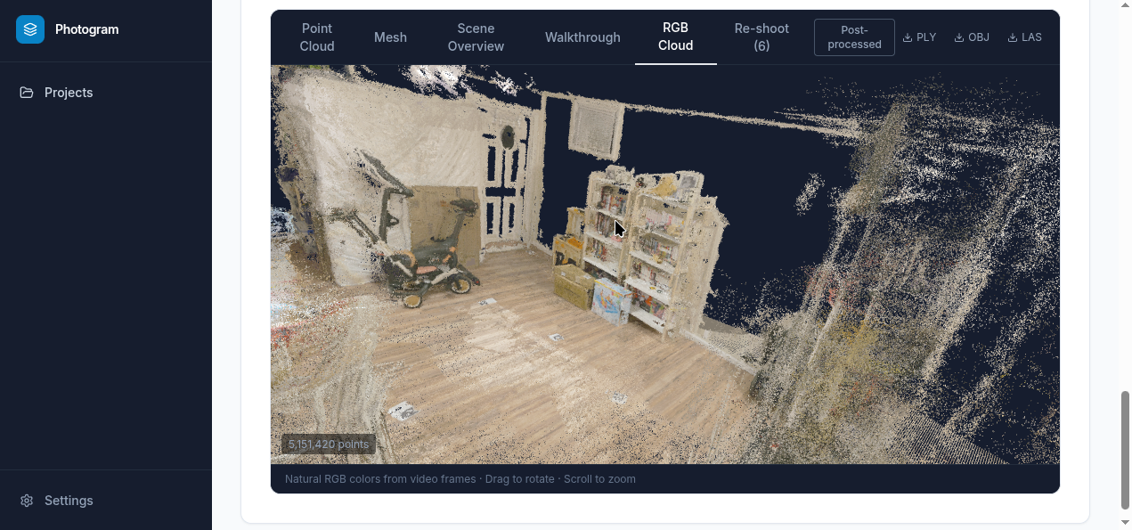
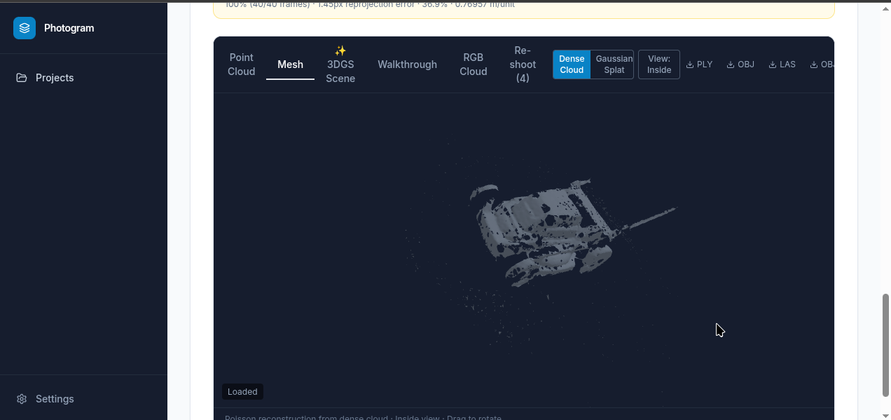
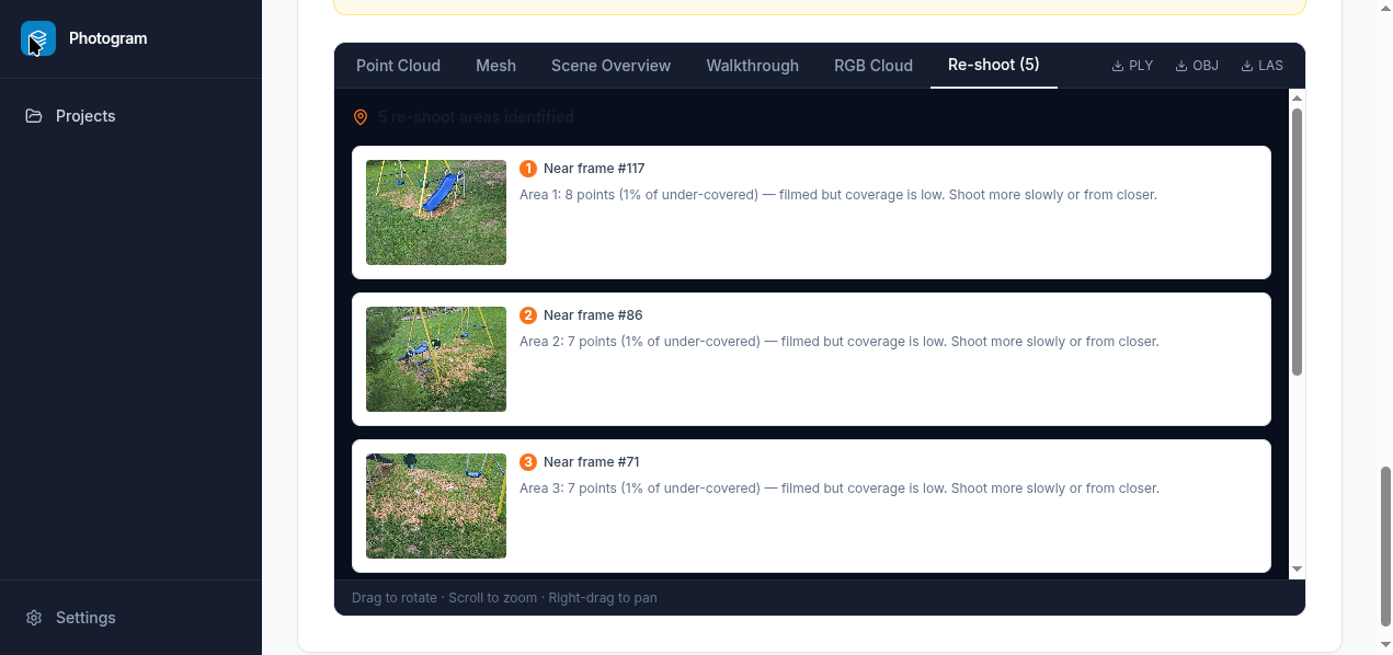
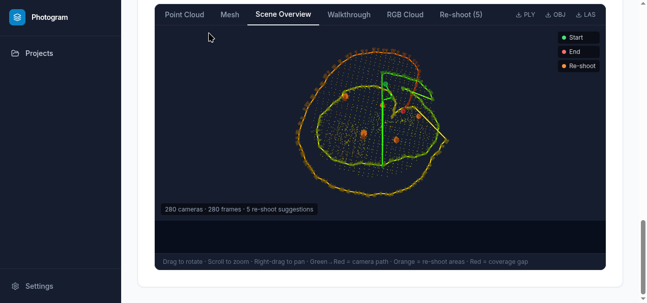
Photogram is a working photogrammetry pipeline and a clean, extensible UI — built not as a product but as a research platform. Three scene modes are supported — indoor room, outdoor survey, and object orbit — each with a separate pipeline branch, mesh algorithm, and coverage boundary. The UI surfaces whatever stages produce: progress tracking with per-stage timings and live GPU telemetry, a 3D viewer with point cloud, mesh, Gaussian splat, scene overview, and camera walkthrough tabs, coverage heatmap, and re-shoot suggestions. Swap a stage, add a new one, and the interface picks it up.
The specific question explored here: where does a vision-language model add real value inside a well-understood classical CV pipeline? Photogrammetry was chosen as the domain because the baseline is solid and well-tooled — feature matching, SfM, and MVS are solved problems. That makes it a good research surface: failures are informative rather than confounded by a weak foundation.
The original target was the two known failure modes of classical MVS — featureless surfaces and thin structures — where VLMs might guide re-sampling or post-processing. A prerequisite step (metric scale) consumed the available experimentation budget. Six VLM integration attempts later, the findings are substantial even if the original question remains open.
If you work in this space and have your own "what if" question — this is a ready-made sandbox. The pipeline is modular, the queue system handles GPU and CPU stages separately, and the UI surfaces whatever your stage produces.
Step through the real SfM camera poses. Rotate freely in place — FOV matched to the recording lens. Blend the original frame over the point cloud or mesh to see exactly where the reconstruction diverges from the real scene. Toggle point cloud ↔ mesh without leaving the camera position.
Six integration attempts across two model tiers (local via Ollama, paid via Gemini) and two phases: first targeting metric scale derivation, then mesh quality improvement. Same wall hit both times. The full research arc — every approach, every failure mode, and what was learned — is documented in docs/journey.md.
Observed consistently across both local and paid models.
The scale problem is fundamentally an information problem, not a perception problem. The video contains no absolute length reference — and rather than trying to extract one post-hoc with AI (unreliable), the right move is to put one in the scene before filming.
ArUco markers are printed squares — standardised in OpenCV, detectable in any lighting, available in dictionaries of up to 1,000 unique IDs. Print them at a known physical size, place them in the scene, film them as part of your walkthrough. The pipeline triangulates each marker's 3D world position from the SfM reconstruction and derives scale from the ratio of known physical distance to SfM-unit distance. With two or more markers co-visible in at least one frame, accuracy is consistently around 2%.
A consistent physical process — print markers, place them, shoot — turned out to be less frustrating, faster, and far more accurate than any AI-based approach. The VLM work was genuinely useful for understanding where the limits are.
14–15 stages, fully automated. Branches by scene_type:
indoor rooms get floor-plane fill and Poisson mesh; outdoor and object scans use Ball Pivoting;
object scans additionally run Gaussian Splatting after MVS.
Fails fast at detect_aruco before any expensive COLMAP stages run.
Outputs: PLY point cloud · OBJ mesh · LAS · .splat for WebGL Gaussian Splat viewer.
%%{init: {'theme': 'base', 'themeVariables': {'fontSize': '15px', 'fontFamily': 'Inter, ui-sans-serif, sans-serif', 'lineColor': '#a5b4fc', 'primaryTextColor': '#e2e4ea', 'primaryColor': '#1e2330', 'primaryBorderColor': '#6366f1', 'secondaryColor': '#252b3b', 'tertiaryColor': '#181c26', 'background': '#0d0f14', 'clusterBkg': '#181c26', 'clusterBorder': '#374151', 'titleColor': '#e2e4ea'}}}%%
flowchart TD
    subgraph extract["Extract (CPU)"]
        A["extract_metadata\nfocal length, GPS, rotation"]
        B["extract_frames\nstep-based, sharpest of burst"]
        C["detect_aruco\nFAIL FAST if no markers"]
        A --> B --> C
    end

    subgraph geometry["Geometry (GPU)"]
        D["feature_matching\nLightGlue + DISK"]
        E["sfm\npycolmap incremental"]
        F["mvs\nCOLMAP patch_match_stereo"]
        D --> E --> F
    end

    subgraph correction["Correction (CPU)"]
        G["correct_trajectory_jumps\nICP fix for teleport blocks"]
    end

    subgraph scale["Scale (CPU)"]
        H["detect_aruco_sfm\nre-scan with COLMAP intrinsics"]
        I["scale_from_aruco\ntriangulate markers → m/unit"]
        J["apply_known_scale\nscale dense cloud to metric"]
        H --> I --> J
    end

    subgraph postprocess["Post-process (CPU)"]
        K["fill_planes\nfloor/wall projection + void fill"]
        L["refine_cloud\nSOR outlier removal + voxel downsample"]
        M["coverage\nHPR + DBSCAN visibility scoring"]
        N["export\nPLY · OBJ · LAS"]
        K --> L --> M --> N
    end

    extract --> geometry --> correction --> scale --> postprocess
target_frames (120–400; more frames if registration was poor), match_window (10–25; wider for better loop closure), and mvs_min_consistent (2–4; tighter when geometry is clean). The full run fires automatically with the calibrated parameters.
POST /api/projects/{"{id}"}/reprocess?from_stage=scale_from_aruco re-runs any downstream stage without re-running COLMAP. Useful when iterating on scale derivation or post-processing after a code change.
Described using the C4 model. The pipeline flowchart above covers the processing detail — these diagrams show how the system is built. Full technical detail including the mesh export pipeline, data model, storage backends, and deployment topology: docs/architecture.md.
Who uses the system and what external dependencies it has. The platform is designed for researchers and engineers who want to experiment with CV and VLM ideas on top of a working photogrammetry baseline.
%%{init: {'theme': 'base', 'themeVariables': {'fontSize': '14px', 'fontFamily': 'Inter, ui-sans-serif, sans-serif', 'lineColor': '#a5b4fc', 'primaryTextColor': '#e2e4ea', 'primaryColor': '#1e2330', 'primaryBorderColor': '#6366f1', 'secondaryColor': '#252b3b', 'tertiaryColor': '#181c26', 'background': '#0d0f14', 'clusterBkg': '#181c26', 'clusterBorder': '#374151', 'titleColor': '#e2e4ea'}}}%%
flowchart TD
    RES(["👤 Researcher / Engineer\nruns scans · reviews 3D output"])

    subgraph platform["Photogram Platform"]
        APP["Photogram\nphotogrammetry pipeline\n& research platform"]
    end

    GPU["⚡ NVIDIA GPU\nCUDA acceleration"]
    HF["🤗 Hugging Face Hub\nLightGlue · nerfstudio weights"]
    STORE["🗄️ Object Storage\nLocal FS · WebDAV · S3"]

    RES -->|"HTTPS + WebSocket"| APP
    APP -->|"CUDA"| GPU
    APP -->|"HTTPS — first use only"| HF
    APP -->|"read/write frames,\nclouds, exports"| STORE
Six deployable containers coordinated by Docker Compose. The GPU and CPU workers consume from separate Celery queues — GPU-bound stages (feature matching, SfM, MVS, Gaussian Splatting) are routed to the GPU worker; everything else goes to the CPU worker. Redis serves triple duty: Celery broker, result backend, and WebSocket pub/sub relay for live pipeline progress.
%%{init: {'theme': 'base', 'themeVariables': {'fontSize': '13px', 'fontFamily': 'Inter, ui-sans-serif, sans-serif', 'lineColor': '#a5b4fc', 'primaryTextColor': '#e2e4ea', 'primaryColor': '#1e2330', 'primaryBorderColor': '#6366f1', 'secondaryColor': '#252b3b', 'tertiaryColor': '#181c26', 'background': '#0d0f14', 'clusterBkg': '#181c26', 'clusterBorder': '#374151', 'titleColor': '#e2e4ea'}}}%%
flowchart TD
    USER(["👤 Researcher"])

    subgraph compose["Docker Compose"]
        FE["Frontend\nNext.js 15 · Three.js\n3D viewer · pipeline monitor\nWebSocket live progress"]
        API["API\nFastAPI · uvicorn\nREST + WebSocket relay\nproject & job management"]
        GPU["GPU Worker\nCelery · CUDA\nfeature matching · SfM\nMVS · Gaussian Splatting"]
        CPU["CPU Worker\nCelery · open3d\nArUco · scale · coverage\nrefine · export"]
        PG[("PostgreSQL\nprojects · jobs · uploads\npipeline_results")]
        REDIS[("Redis\nCelery broker\nresult backend\nWebSocket pub/sub")]
        STORE[("Storage\nLocal FS / S3 / WebDAV\nframes · clouds · exports")]
    end

    USER -->|"HTTPS"| FE
    FE -->|"REST + WS"| API
    API -->|"asyncpg"| PG
    API -->|"pub/sub"| REDIS
    API -->|"Celery task"| GPU
    API -->|"Celery task"| CPU
    GPU -->|"progress"| REDIS
    CPU -->|"progress"| REDIS
    GPU <-->|"read/write"| STORE
    CPU <-->|"read/write"| STORE
    FE <-->|"WS relay"| REDIS
The major modules inside the two Celery workers. Each pipeline stage is a self-contained module under backend/workers/pipeline/ — it receives prev_result, does its work, updates prev_result, and returns it. The Celery task wrapper in tasks.py handles job tracking, heartbeats, progress events, and cleanup. Neither layer knows about the other's concerns.
%%{init: {'theme': 'base', 'themeVariables': {'fontSize': '13px', 'fontFamily': 'Inter, ui-sans-serif, sans-serif', 'lineColor': '#a5b4fc', 'primaryTextColor': '#e2e4ea', 'primaryColor': '#1e2330', 'primaryBorderColor': '#6366f1', 'secondaryColor': '#252b3b', 'tertiaryColor': '#181c26', 'background': '#0d0f14', 'clusterBkg': '#181c26', 'clusterBorder': '#374151', 'titleColor': '#e2e4ea'}}}%%
flowchart TB
    subgraph gpu["⚡ GPU Worker (gpu queue)"]
        direction LR
        FM["feature_matching\nLightGlue + DISK"] --> SFM["sfm\npycolmap"] --> MVS["mvs\nCOLMAP CUDA"] --> GS["gaussian_splatting\nnerfstudio · object only"]
    end

    subgraph cpu["🖥️ CPU Worker (celery queue)"]
        direction LR
        EM["extract_metadata"] --> EF["extract_frames"] --> AD["detect_aruco"] --> TC["correct_trajectory"] --> AS["detect_aruco_sfm"] --> SF["scale_from_aruco"] --> AK["apply_scale"] --> FP["fill_planes"] --> RC["refine_cloud"] --> COV["coverage"] --> EXP["export"]
    end

    gpu --> cpu
Three patterns that hold the system together: the Celery chain that wires stages into a pipeline, the WebSocket relay that surfaces live progress to the frontend, and the reprocess checkpoint that lets any post-SfM stage be re-run without repeating the hours-long COLMAP stages.
%%{init: {'theme': 'base', 'themeVariables': {'fontSize': '13px', 'fontFamily': 'Inter, ui-sans-serif, sans-serif', 'lineColor': '#a5b4fc', 'primaryTextColor': '#e2e4ea', 'primaryColor': '#1e2330', 'primaryBorderColor': '#6366f1', 'secondaryColor': '#252b3b', 'tertiaryColor': '#181c26', 'background': '#0d0f14', 'clusterBkg': '#181c26', 'clusterBorder': '#374151', 'titleColor': '#e2e4ea'}}}%%
flowchart TB
    subgraph row1[" "]
        direction LR
        subgraph chain["Celery chain — pipeline dispatch"]
            direction LR
            C1["extract_metadata\nextract_frames\ndetect_aruco"] --> C2["GPU stages\nfeature · sfm · mvs"] --> C3["detect_aruco_sfm"] -->|"checkpoint → Redis"| C4["scale_from_aruco\napply_scale · refine · export"]
        end
        subgraph ws["WebSocket — live progress"]
            direction LR
            W1["publish_progress()\nin each stage"] --> W2["Redis\npub/sub"] --> W3["API WS\nrelay"] --> W4["Browser\nlive update"]
        end
    end

    subgraph row2[" "]
        direction LR
        subgraph reprocess["POST /reprocess — partial re-run"]
            direction LR
            R1["read checkpoint\nfrom Redis"] --> R2["dispatch chain\nfrom any stage"] --> R3["minutes not hours\nno COLMAP re-run"]
        end
        subgraph emit["emit_stage_complete — persistence"]
            direction LR
            E1["stage\nfinishes"] --> E2["WS event +\nDB write"] --> E3["pipeline_results\nmetrics · timings"] --> E4["page reload\nno WS needed"]
        end
    end

    row1 --> row2

    style row1 fill:none,stroke:none
    style row2 fill:none,stroke:none